At this time, people all over the world are fighting with the Covid-19 pandemic, which has been causing a global public health emergency. Due to the new variations, the number of infected people is increasing everyday, which puts tremendous pressure on the healthcare system. An automated system to detect visual indicators of Covid-19 is therefore needed. In this blog post, we attempt to use deep learning to detect Covid infection on X-ray images. Note that this is only a showcase for the application of deep learning on real-world scenario, and the model presented here can no way replace medical professionals. Nevertheless, the model might be useful to classify and visualize segments of images that can be related to a Covid infection.
Dataset and Dataloaders
We are going to use the Covid-19 Image Dataset for our task. The dataset contains labeled X-ray image data from 3 classes: Normal, Covid-19, and Viral Pneumonia (infection of your lungs caused by a virus. This causes inflammation in the tiny air sacs inside your lungs that make it hard to breathe).
Let’s first import the required packages
import os
import random

import numpy as np
import pandas as pd
import scipy as sp
import matplotlib.pyplot as plt
import cv2
from sklearn.model_selection import train_test_split
from sklearn.metrics import classification_report, accuracy_score, confusion_matrix

import tensorflow as tf
from tensorflow.keras.models import *
from tensorflow.keras.layers import *
from tensorflow.keras.optimizers import *
from tensorflow.keras.applications import vgg16
from tensorflow.keras.preprocessing.image import img_to_array, array_to_img, ImageDataGenerator
We will crop the data to uniform size so that they can be processed parallelly as tensors
base_path = "/content/infection_imgs/Covid19-dataset"
HEIGHT = 224
WIDTH = 224
BATCH_SIZE = 32
SEED = 42
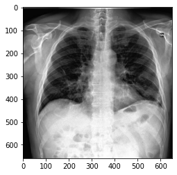
Visualize a single image:
img = cv2.imread("/content/infection_imgs/Covid19-dataset/test/Covid/0100.jpeg")
plt.imshow(img)

The next step is to define the Data Generators. We add some random augmentation steps to the training data to avoid overfitting and encourage the model to learn the relevant features:
train_generator = ImageDataGenerator(rescale=1/255,
                                rotation_range=10, # rotation
                                width_shift_range=0.2, # horizontal shift
                                height_shift_range=0.2, # vertical shift
                                zoom_range=0.2, # zoom
                                brightness_range=[0.2,1.2])
test_generator = ImageDataGenerator(rescale=1/255)
Then we collect the data from the folders:
train_generator = train_generator.flow_from_directory(
            os.path.join(base_path, "train"),
            target_size = (HEIGHT,WIDTH),
            batch_size = BATCH_SIZE,
            class_mode = 'categorical',
            shuffle = True,
            seed = SEED
)

test_generator = test_generator.flow_from_directory(
            os.path.join(base_path, "test"),
            target_size = (HEIGHT,WIDTH),
            batch_size = BATCH_SIZE,
            class_mode = 'categorical',
            shuffle = True,
            seed = SEED
)
Found 251 images belonging to 3 classes.
Found 66 images belonging to 3 classes.
Define the model
We will not train the model from scratch, rather employ deep transfer learning techniques. To be precise, we employ the pretrained model VGG16 for our task, freezing the beginning blocks and only train the last two convolutional blocks for the features extraction. Besides, we add a https://alexisbcook.github.io/2017/global-average-pooling-layers-for-object-localization/, which is capable of extreme dimensionality reduction, to avoid overfitting.
vgg = vgg16.VGG16(weights='imagenet', include_top=False, input_shape = (HEIGHT,WIDTH, 3))

# freeze
for layer in vgg.layers[:-8]:
    layer.trainable = False

x = vgg.output
# reduce size of previous layer by taking average of each feature map to avoid overfitting
x = GlobalAveragePooling2D()(x)
x = Dense(3, activation="softmax")(x)

model = Model(vgg.input, x)
model.compile(loss = "categorical_crossentropy",
              optimizer = SGD(learning_rate=3e-3, momentum=0.9), metrics=["accuracy"])
model.summary()
Model: "model"
_________________________________________________________________
 Layer (type)                Output Shape              Param #
=================================================================
 input_1 (InputLayer)        [(None, 224, 224, 3)]     0

 block1_conv1 (Conv2D)       (None, 224, 224, 64)      1792

 block1_conv2 (Conv2D)       (None, 224, 224, 64)      36928

 block1_pool (MaxPooling2D)  (None, 112, 112, 64)      0

 block2_conv1 (Conv2D)       (None, 112, 112, 128)     73856

 block2_conv2 (Conv2D)       (None, 112, 112, 128)     147584

 block2_pool (MaxPooling2D)  (None, 56, 56, 128)       0

 block3_conv1 (Conv2D)       (None, 56, 56, 256)       295168

 block3_conv2 (Conv2D)       (None, 56, 56, 256)       590080

 block3_conv3 (Conv2D)       (None, 56, 56, 256)       590080

 block3_pool (MaxPooling2D)  (None, 28, 28, 256)       0

 block4_conv1 (Conv2D)       (None, 28, 28, 512)       1180160

 block4_conv2 (Conv2D)       (None, 28, 28, 512)       2359808

 block4_conv3 (Conv2D)       (None, 28, 28, 512)       2359808

 block4_pool (MaxPooling2D)  (None, 14, 14, 512)       0

 block5_conv1 (Conv2D)       (None, 14, 14, 512)       2359808

 block5_conv2 (Conv2D)       (None, 14, 14, 512)       2359808

 block5_conv3 (Conv2D)       (None, 14, 14, 512)       2359808

 block5_pool (MaxPooling2D)  (None, 7, 7, 512)         0

 global_average_pooling2d (G  (None, 512)              0
 lobalAveragePooling2D)

 dense (Dense)               (None, 3)                 1539

=================================================================
Total params: 14,716,227
Trainable params: 12,980,739
Non-trainable params: 1,735,488
_________________________________________________________________
Now as we are all set, we can start training the model:
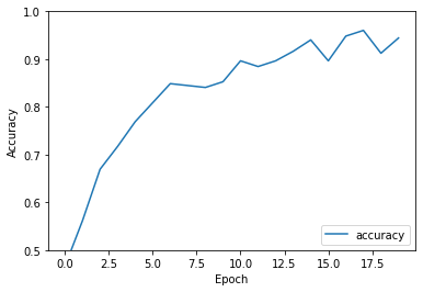
history = model.fit(train_generator, steps_per_epoch=train_generator.samples/train_generator.batch_size, epochs=20)
Epoch 1/20
7/7 [==============================] - 18s 2s/step - loss: 1.0410 - accuracy: 0.4661
Epoch 2/20
7/7 [==============================] - 15s 2s/step - loss: 0.9330 - accuracy: 0.5618
Epoch 3/20
7/7 [==============================] - 15s 2s/step - loss: 0.7757 - accuracy: 0.6693
Epoch 4/20
7/7 [==============================] - 15s 2s/step - loss: 0.6472 - accuracy: 0.7171
Epoch 5/20
7/7 [==============================] - 16s 2s/step - loss: 0.5488 - accuracy: 0.7689
Epoch 6/20
7/7 [==============================] - 15s 2s/step - loss: 0.4505 - accuracy: 0.8088
Epoch 7/20
7/7 [==============================] - 17s 2s/step - loss: 0.3590 - accuracy: 0.8486
Epoch 8/20
7/7 [==============================] - 22s 3s/step - loss: 0.3644 - accuracy: 0.8446
Epoch 9/20
7/7 [==============================] - 15s 2s/step - loss: 0.3517 - accuracy: 0.8406
Epoch 10/20
7/7 [==============================] - 15s 2s/step - loss: 0.3075 - accuracy: 0.8526
Epoch 11/20
7/7 [==============================] - 15s 2s/step - loss: 0.2827 - accuracy: 0.8964
Epoch 12/20
7/7 [==============================] - 17s 2s/step - loss: 0.2936 - accuracy: 0.8845
Epoch 13/20
7/7 [==============================] - 20s 2s/step - loss: 0.2952 - accuracy: 0.8964
Epoch 14/20
7/7 [==============================] - 15s 2s/step - loss: 0.2275 - accuracy: 0.9163
Epoch 15/20
7/7 [==============================] - 14s 2s/step - loss: 0.1597 - accuracy: 0.9402
Epoch 16/20
7/7 [==============================] - 14s 2s/step - loss: 0.2454 - accuracy: 0.8964
Epoch 17/20
7/7 [==============================] - 14s 2s/step - loss: 0.1714 - accuracy: 0.9482
Epoch 18/20
7/7 [==============================] - 15s 2s/step - loss: 0.1167 - accuracy: 0.9602
Epoch 19/20
7/7 [==============================] - 15s 2s/step - loss: 0.1855 - accuracy: 0.9124
Epoch 20/20
7/7 [==============================] - 14s 2s/step - loss: 0.1325 - accuracy: 0.9442
plt.plot(history.history['accuracy'], label='accuracy')
plt.xlabel('Epoch')
plt.ylabel('Accuracy')
plt.ylim([0.5, 1])
plt.legend(loc='lower right')
<matplotlib.legend.Legend at 0x7f3b0f262e50>

Model Evaluation
We can evaluate the model performance on the test set:
test_loss_ = []
test_acc_ = []
i = 0

for test_images,  test_labels in test_generator:
  test_loss, test_acc = model.evaluate(test_images,  test_labels, verbose=2)
  test_loss_.append(test_loss)
  test_acc_.append(test_acc)
  i += 1
  if (i == 3): break
np.mean(test_loss_), np.mean(test_acc_)
1/1 - 0s - loss: 0.2964 - accuracy: 0.9375 - 263ms/epoch - 263ms/step
1/1 - 0s - loss: 0.2800 - accuracy: 1.0000 - 92ms/epoch - 92ms/step
1/1 - 0s - loss: 0.1836 - accuracy: 0.9375 - 257ms/epoch - 257ms/step


(0.25333257019519806, 0.9583333333333334)
Our model achieved an accuracy of 96%, which might indicate a good model.
predicted = []
real = []
for X, y in test_generator:
  real.extend(np.argmax(y,axis=1))
  predicted.extend(np.argmax(model.predict(X),axis=1))
  break
We can also use the classification_report method of scikit-learn to look at other evaluation metrics:
print(classification_report(real, predicted))
              precision    recall  f1-score   support

           0       1.00      0.94      0.97        16
           1       0.80      1.00      0.89         8
           2       1.00      0.88      0.93         8

    accuracy                           0.94        32
   macro avg       0.93      0.94      0.93        32
weighted avg       0.95      0.94      0.94        32
test_generator.class_indices
{'Covid': 0, 'Normal': 1, 'Viral Pneumonia': 2}
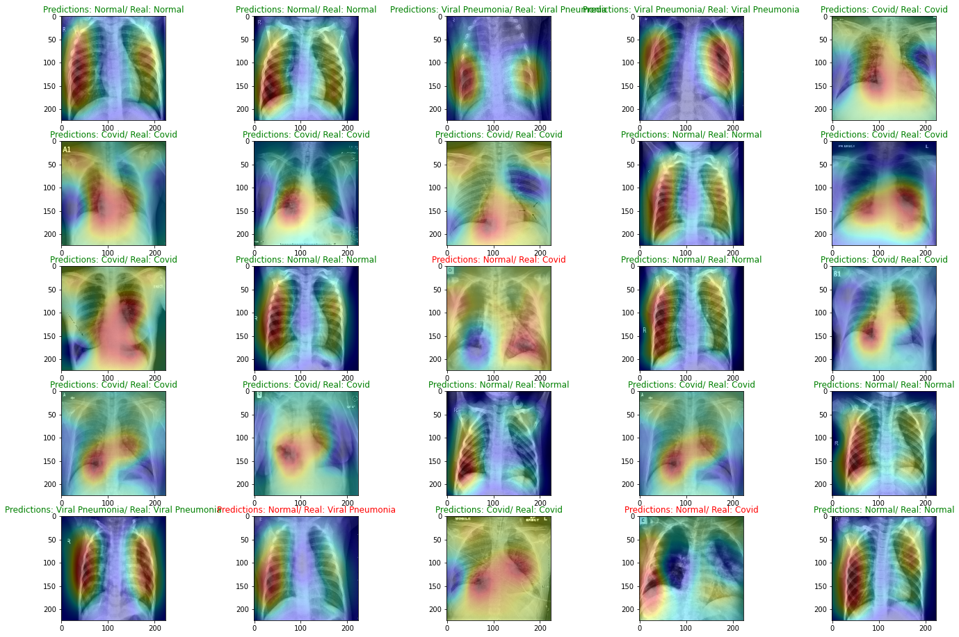
Another great feature of Global Average Pooling is that CNNs with GAP layers that have been trained for a classification task can also be used for object localization! It not only classifies the image, but also WHERE the evidences are located. Therefore, we can create a heat map representation for such models. This is don by a bilinear upsampling of the activation map to the training image size.
The function below defines this visualization:
cs = ['Covid', 'Normal',  'Viral Pneumonia']
# adapt from https://github.com/cerlymarco/MEDIUM_NoteBook/blob/master/Anomaly_Detection_Image/Anomaly_Detection_Image.ipynb
def plot_activation(img, i, label):
    pred_class = np.argmax(model.predict(img[np.newaxis,:,:,:]))

    weights = model.layers[-1].get_weights()[0]
    class_weights = weights[:, pred_class]

    intermediate = Model(model.input, model.get_layer("block5_conv3").output)
    conv_output = np.squeeze(intermediate.predict(img[np.newaxis,:,:,:]))

    h = int(img.shape[0]/conv_output.shape[0])
    w = int(img.shape[1]/conv_output.shape[1])

    activation_maps = sp.ndimage.zoom(conv_output, (h, w, 1), order=1)
   # print(conv_output.shape, h, w, activation_maps.shape, img.shape[0],img.shape[1])
    out = np.dot(activation_maps.reshape((img.shape[0]*img.shape[1], 512)), class_weights).reshape(img.shape[0],img.shape[1])

    plt.subplot(5,5,i)
    plt.imshow(img.astype('float32').reshape(img.shape[0],img.shape[1],3))
    plt.imshow(out, cmap='jet', alpha=0.35)
    label = np.argmax(label)
    if cs[pred_class]  != cs[label]:
       plt.title("Predictions: " + cs[pred_class] + "/ Real: " + cs[label], color = "red")
    else:
      plt.title("Predictions: " + cs[pred_class] + "/ Real: " + cs[label], color = "green")
plt.figure(figsize=(24,16))
imgs, label = next(iter(test_generator))
print(imgs.shape)
for i in range(25):
  img_ = plot_activation(imgs[i], i+1, label[i])
(32, 224, 224, 3)

Surprisingly, the model does a good job on detecting Covid infection: it highlights the ground-glass opacities in the images, which is a clear indicator for a Covid infection, see here.
Conclusion
We have trained a model for Covid 19 detection and visualization. The model achieved a precision of 96% and can learn the part of the images that are important for Covid detection. Note that the dataset employed here is quite small, so a larger and more curated dataset might help improve the model performance.


