Introduction

This blog post attempts to study the factors that influence the sale price of houses. To be specific, we will study the Ames Housing dataset , which can be downloaded from Kaggle.

import datetime
import random
import os 

import numpy as np
import pandas as pd
import seaborn as sns
import matplotlib.pyplot as plt

from sklearn.kernel_ridge import KernelRidge
from sklearn.linear_model import Ridge, RidgeCV, ElasticNet, ElasticNetCV
from sklearn.svm import SVR
from sklearn.model_selection import GridSearchCV, KFold, cross_val_score, train_test_split
from sklearn.metrics import mean_squared_error
from sklearn.preprocessing import OneHotEncoder, LabelEncoder, scale
from sklearn.preprocessing import StandardScaler, RobustScaler
from sklearn.ensemble import RandomForestRegressor, GradientBoostingRegressor
from sklearn.pipeline import make_pipeline
from sklearn.decomposition import PCA

from scipy.special import boxcox1p
from scipy.stats import boxcox_normmax

from mlxtend.regressor import StackingCVRegressor
import lightgbm as lgb
from lightgbm import LGBMRegressor
from xgboost import XGBRegressor

Data Preprocessing and Exploring

The goal of this notebook is to predict SalePrice of houses

train_data = pd.read_csv('data/train.csv')
test_data = pd.read_csv('data/test.csv')
train_data.shape, test_data.shape

((1460, 81), (1459, 80))

train_data.head()

	Id	MSSubClass	MSZoning	LotFrontage	LotArea	Street	Alley	LotShape	LandContour	Utilities	LotConfig	LandSlope	Neighborhood	Condition1	Condition2	BldgType	HouseStyle	OverallQual	OverallCond	YearBuilt	YearRemodAdd	RoofStyle	RoofMatl	Exterior1st	Exterior2nd	MasVnrType	MasVnrArea	ExterQual	ExterCond	Foundation	BsmtQual	BsmtCond	BsmtExposure	BsmtFinType1	BsmtFinSF1	BsmtFinType2	BsmtUnfSF	TotalBsmtSF	Heating	...	CentralAir	Electrical	1stFlrSF	2ndFlrSF	GrLivArea	BsmtFullBath	BsmtHalfBath	FullBath	HalfBath	BedroomAbvGr	KitchenAbvGr	KitchenQual	TotRmsAbvGrd	Functional	Fireplaces	FireplaceQu	GarageType	GarageYrBlt	GarageFinish	GarageCars	GarageArea	GarageQual	GarageCond	PavedDrive	WoodDeckSF	OpenPorchSF	EnclosedPorch	PoolQC	Fence	MiscFeature	MoSold	YrSold	SaleType	SaleCondition	SalePrice
0	1	60	RL	65.0	8450	Pave	NaN	Reg	Lvl	AllPub	Inside	Gtl	CollgCr	Norm	Norm	1Fam	2Story	7	5	2003	2003	Gable	CompShg	VinylSd	VinylSd	BrkFace	196.0	Gd	TA	PConc	Gd	TA	No	GLQ	706	Unf	150	856	GasA	...	Y	SBrkr	856	854	1710	1	0	2	1	3	1	Gd	8	Typ	0	NaN	Attchd	2003.0	RFn	2	548	TA	TA	Y	0	61	0	NaN	NaN	NaN	2	2008	WD	Normal	208500
1	2	20	RL	80.0	9600	Pave	NaN	Reg	Lvl	AllPub	FR2	Gtl	Veenker	Feedr	Norm	1Fam	1Story	6	8	1976	1976	Gable	CompShg	MetalSd	MetalSd	None	0.0	TA	TA	CBlock	Gd	TA	Gd	ALQ	978	Unf	284	1262	GasA	...	Y	SBrkr	1262	0	1262	0	1	2	0	3	1	TA	6	Typ	1	TA	Attchd	1976.0	RFn	2	460	TA	TA	Y	298	0	0	NaN	NaN	NaN	5	2007	WD	Normal	181500
2	3	60	RL	68.0	11250	Pave	NaN	IR1	Lvl	AllPub	Inside	Gtl	CollgCr	Norm	Norm	1Fam	2Story	7	5	2001	2002	Gable	CompShg	VinylSd	VinylSd	BrkFace	162.0	Gd	TA	PConc	Gd	TA	Mn	GLQ	486	Unf	434	920	GasA	...	Y	SBrkr	920	866	1786	1	0	2	1	3	1	Gd	6	Typ	1	TA	Attchd	2001.0	RFn	2	608	TA	TA	Y	0	42	0	NaN	NaN	NaN	9	2008	WD	Normal	223500
3	4	70	RL	60.0	9550	Pave	NaN	IR1	Lvl	AllPub	Corner	Gtl	Crawfor	Norm	Norm	1Fam	2Story	7	5	1915	1970	Gable	CompShg	Wd Sdng	Wd Shng	None	0.0	TA	TA	BrkTil	TA	Gd	No	ALQ	216	Unf	540	756	GasA	...	Y	SBrkr	961	756	1717	1	0	1	0	3	1	Gd	7	Typ	1	Gd	Detchd	1998.0	Unf	3	642	TA	TA	Y	0	35	272	NaN	NaN	NaN	2	2006	WD	Abnorml	140000
4	5	60	RL	84.0	14260	Pave	NaN	IR1	Lvl	AllPub	FR2	Gtl	NoRidge	Norm	Norm	1Fam	2Story	8	5	2000	2000	Gable	CompShg	VinylSd	VinylSd	BrkFace	350.0	Gd	TA	PConc	Gd	TA	Av	GLQ	655	Unf	490	1145	GasA	...	Y	SBrkr	1145	1053	2198	1	0	2	1	4	1	Gd	9	Typ	1	TA	Attchd	2000.0	RFn	3	836	TA	TA	Y	192	84	0	NaN	NaN	NaN	12	2008	WD	Normal	250000

5 rows × 81 columns

Next, we would like to understand the correlation between the target and other numerical features:

corrmat = train_data.corr()
f, ax = plt.subplots(figsize=(8, 6))
sns.heatmap(corrmat, vmax=.8, square=True)

png

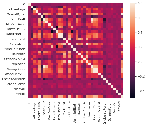
Next, we study the top 10 features that has the highest correlation to the target:

k = 10
cols = corrmat.nlargest(k, 'SalePrice')['SalePrice'].index
cm = np.corrcoef(train_data[cols].values.T)
sns.set(font_scale=1.25)
plt.subplots(figsize=(8, 6))
sns.heatmap(cm, cbar=True, annot=True, square=True, fmt='.2f', annot_kws={'size': 10}, yticklabels=cols.values, xticklabels=cols.values)

<matplotlib.axes._subplots.AxesSubplot at 0x7f3014d93d10>

png

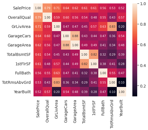
Following points can be infered from the heatmap:

‘OverallQual’ (Overall material and finish quality ), ‘GrLivArea’ (Above grade (ground) living area square feet) and ‘TotalBsmtSF’ (Total square feet of basement area) are strongly correlated with ‘SalePrice’, which totally makes sense
2 next highly collerated features are ‘GarageCars’ (Size of garage in car capacity) and ‘GarageArea’ (Size of garage in square feet). It is noteworthy that these two features indicate quite similar characteristics; indeed, ‘GarageCars’ is a consequence of ‘GarageArea’. The same applies to ‘TotalBsmtSF’ (Total square feet of basement area) and ‘1stFloor’

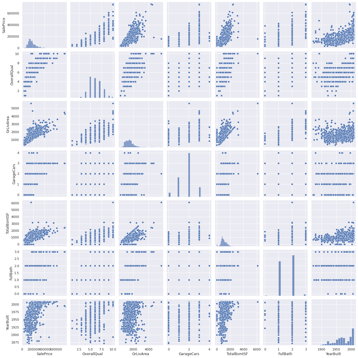
Next, we take a closer look to 5 intereseting features.

sns.set()
cols = ['SalePrice', 'OverallQual', 'GrLivArea', 'GarageCars', 'TotalBsmtSF', 'FullBath', 'YearBuilt']
sns.pairplot(train_data[cols], size = 2.5)
plt.show();

/usr/local/lib/python3.7/dist-packages/seaborn/axisgrid.py:2076: UserWarning: The `size` parameter has been renamed to `height`; please update your code.
  warnings.warn(msg, UserWarning)

png

Subsequently, we would like to study the data on missing data:

total = train_data.isnull().sum().sort_values(ascending=False)
percent = (train_data.isnull().sum()/train_data.isnull().count()).sort_values(ascending=False)
missing_data = pd.concat([total, percent], axis=1, keys=['Total', 'Percent'])
missing_data.head(20)

	Total	Percent
PoolQC	1453	0.995205
MiscFeature	1406	0.963014
Alley	1369	0.937671
Fence	1179	0.807534
FireplaceQu	690	0.472603
LotFrontage	259	0.177397
GarageCond	81	0.055479
GarageType	81	0.055479
GarageYrBlt	81	0.055479
GarageFinish	81	0.055479
GarageQual	81	0.055479
BsmtExposure	38	0.026027
BsmtFinType2	38	0.026027
BsmtFinType1	37	0.025342
BsmtCond	37	0.025342
BsmtQual	37	0.025342
MasVnrArea	8	0.005479
MasVnrType	8	0.005479
Electrical	1	0.000685
Utilities	0	0.000000

There are several features that are mostly missed (> 80%). Since these features are not what we will consider when buying a house, we can safely drop them. Next, ‘FireplaceQu’ is something quite subjective and might be a source for outliers, so we also drop it.

Next, the ‘Garage…’ features seem to refer to the same phenomena, and they are actually highly related to ‘GarageCars’, therefore, they are safe to delete. The same applies to ‘Bsmt…’ features, which are related to ‘TotalBsmtSF’. Both ‘TotalBsmtSF’ and ‘GarageCars’ have been already considered.

The rest 3 features ‘MasVnrArea’ (Masonry veneer area in square feet), ‘MasVnrType’ (Masonry veneer type) and ‘Electrical’ (Electrical system) are 3 characteristics that do not really go into house price and can be replaced by the housebuyers, so we can drop these columns without losing much information. Besides, ‘MasVnrArea’ and ‘MasVnrType’ can be infered from ‘OverallQual’

train_data = train_data.drop((missing_data[missing_data['Total'] >= 1]).index,1)
train_data.isnull().sum().max() # check if all missing columns are handled

Next, we would like to see how the target is distributed

sns.set_style("white")
f, ax = plt.subplots(figsize=(8, 6))
sns.histplot(train_data['SalePrice'], color="b", kde=True, stat="density")
ax.set(title="SalePrice distribution")
sns.despine(trim=True, left=True)

png

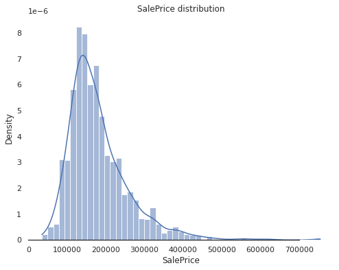
As in the plot, the SalePrice distribution is skewed from the normal distribution and shows peakedness. These values can be obtained as follows:

print("Skewness: %f" % train_data['SalePrice'].skew()) # skewness
print("Kurtosis: %f" % train_data['SalePrice'].kurt()) # deviation from the normal distribution

Skewness: 1.882876
Kurtosis: 6.536282

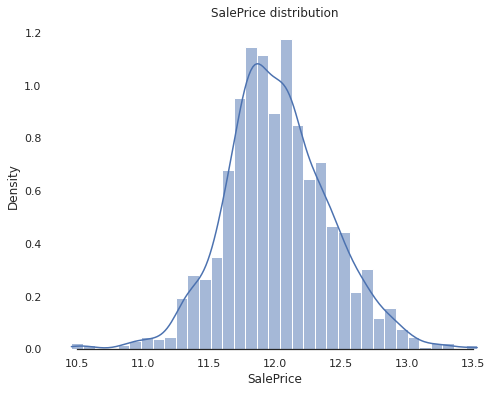
Since most ML models cannot handle non-normally distributed data very well, we should scale the feature appropriately. Recall that log transformation log(1+x) can fix the positive skewness. We apply this to the data and verified the transformed feature:

train_data["SalePrice"] = np.log1p(train_data["SalePrice"])

sns.set_style("white")
f, ax = plt.subplots(figsize=(8, 6))
sns.histplot(train_data['SalePrice'], color="b", kde=True, stat="density")
ax.set(title="SalePrice distribution")
sns.despine(trim=True, left=True)

png

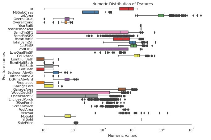
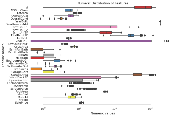
In the next step, we would like to fix skewed numerical features. The first thing to do is to create box plots for these features:

# get numeric columns
numerics = ['int16', 'int32', 'int64', 'float16', 'float32', 'float64']
numeric_data = train_data.select_dtypes(include=numerics)

# Create box plots for all numeric features
sns.set_style("white")
f, ax = plt.subplots(figsize=(10, 7))
ax.set_xscale("log")
ax = sns.boxplot(data=numeric_data , orient="h", palette="Set1")
ax.xaxis.grid(False)
ax.set(ylabel="Feature names")
ax.set(xlabel="Numeric values")
ax.set(title="Numeric Distribution of Features")
sns.despine(trim=True, left=True)

png

# Find skewed numerical features
skew_features = numeric_data.apply(lambda x: x.skew()).sort_values(ascending=False)

high_skew = skew_features[skew_features > 0.5]
skew_index = high_skew.index

print("There are {} numerical features with Skew > 0.5 :".format(high_skew.shape[0]))
skewness = pd.DataFrame({'Skew' :high_skew})
skew_features.keys()

There are 24 numerical features with Skew > 0.5 :





Index(['MiscVal', 'PoolArea', 'LotArea', '3SsnPorch', 'LowQualFinSF',
       'KitchenAbvGr', 'BsmtFinSF2', 'ScreenPorch', 'BsmtHalfBath',
       'EnclosedPorch', 'OpenPorchSF', 'BsmtFinSF1', 'WoodDeckSF',
       'TotalBsmtSF', 'MSSubClass', '1stFlrSF', 'GrLivArea', 'BsmtUnfSF',
       '2ndFlrSF', 'OverallCond', 'TotRmsAbvGrd', 'HalfBath', 'Fireplaces',
       'BsmtFullBath', 'OverallQual', 'MoSold', 'BedroomAbvGr', 'GarageArea',
       'SalePrice', 'YrSold', 'FullBath', 'Id', 'GarageCars', 'YearRemodAdd',
       'YearBuilt'],
      dtype='object')

We employ the Box-Cox transformation to normalize the skewed features

for i in skew_index:
    train_data[i] = boxcox1p(train_data[i], boxcox_normmax(train_data[i] + 1))

/usr/local/lib/python3.7/dist-packages/scipy/stats/stats.py:3508: PearsonRConstantInputWarning: An input array is constant; the correlation coefficent is not defined.
  warnings.warn(PearsonRConstantInputWarning())
/usr/local/lib/python3.7/dist-packages/scipy/stats/stats.py:3538: PearsonRNearConstantInputWarning: An input array is nearly constant; the computed correlation coefficent may be inaccurate.
  warnings.warn(PearsonRNearConstantInputWarning())

numeric_data = train_data.select_dtypes(include=numerics)
# Create box plots for all numeric features
sns.set_style("white")
f, ax = plt.subplots(figsize=(10, 7))
ax.set_xscale("log")
ax = sns.boxplot(data=numeric_data , orient="h", palette="Set1")
ax.xaxis.grid(False)
ax.set(ylabel="Feature names")
ax.set(xlabel="Numeric values")
ax.set(title="Numeric Distribution of Features")
sns.despine(trim=True, left=True)

png

In the following, we encode and embed categorical feature:

# select categorical feazires
categorical_features = train_data.select_dtypes(include = ["object"]).columns
train_cat = train_data[categorical_features]
# one-hot encoding
train_cat = pd.get_dummies(train_cat)
train_cat.head()

	MSZoning_RL	Street_Pave	LotShape_IR1	LotShape_Reg	LandContour_Lvl	Utilities_AllPub	LotConfig_Corner	LotConfig_FR2	LotConfig_Inside	LandSlope_Gtl	Neighborhood_CollgCr	Neighborhood_Crawfor	...	HeatingQC_Ex	HeatingQC_Gd	CentralAir_Y	KitchenQual_Gd	KitchenQual_TA	Functional_Typ	PavedDrive_Y	SaleType_WD	SaleCondition_Abnorml	SaleCondition_Normal
0	1	1	0	1	1	1	0	0	1	1	1	0	...	1	0	1	1	0	1	1	1	0	1
1	1	1	0	1	1	1	0	1	0	1	0	0	...	1	0	1	0	1	1	1	1	0	1
2	1	1	1	0	1	1	0	0	1	1	1	0	...	1	0	1	1	0	1	1	1	0	1
3	1	1	1	0	1	1	1	0	0	1	0	1	...	0	1	1	1	0	1	1	1	1	0
4	1	1	1	0	1	1	0	1	0	1	0	0	...	1	0	1	1	0	1	1	1	0	1

5 rows × 182 columns

# join numerical and categorical columns
train_data_preprocess = pd.concat([numeric_data, train_cat], axis = 1)
train_target = train_data_preprocess['SalePrice']
train_features = train_data_preprocess.drop('SalePrice', axis=1)
X_train, X_test, y_train, y_test = train_test_split(train_features, train_target, test_size = 0.3, random_state = 0)
X_train.shape, X_test.shape, y_train.shape, y_test.shape

((1022, 216), (438, 216), (1022,), (438,))

Next, we do the standardation separately for the training and test set. Note that we must not fit the StandardScaler on observations that are later used for testing

stdSc = StandardScaler()
numerical_features = X_train.select_dtypes(include=numerics).columns
X_train.loc[:, numerical_features] = stdSc.fit_transform(X_train.loc[:, numerical_features])
X_test.loc[:, numerical_features] = stdSc.transform(X_test.loc[:, numerical_features])

Model Definition

In this section, we train several models on the preprocessed datasets. The first step is to define a k-cross validator and the metrics:

# Setup cross validation folds
kf = KFold(n_splits=12, random_state=42, shuffle=True)

def rmsle(y, y_pred):
    return np.sqrt(mean_squared_error(y, y_pred))

def cv_rmse(model, X=X_test, y=y_test):
    rmse = np.sqrt(-cross_val_score(model, X, y, scoring="neg_mean_squared_error", cv=kf))
    return rmse

# elastic net
from sklearn.linear_model import ElasticNet
elastic_net = ElasticNet(alpha=0.1, l1_ratio=0.5, random_state=42)

ElasticNet(alpha=0.1, random_state=42)

# Light Gradient Boosting Regressor
lightgbm = LGBMRegressor(objective='regression', 
                       num_leaves=6,
                       learning_rate=0.01, 
                       n_estimators=7000,
                       max_bin=200, 
                       bagging_fraction=0.8,
                       bagging_freq=4, 
                       bagging_seed=8,
                       feature_fraction=0.2,
                       feature_fraction_seed=8,
                       min_sum_hessian_in_leaf = 11,
                       verbose=-1,
                       random_state=42)

# XGBoost Regressor
xgboost = XGBRegressor(learning_rate=0.01,
                       n_estimators=6000,
                       max_depth=4,
                       min_child_weight=0,
                       gamma=0.6,
                       subsample=0.7,
                       colsample_bytree=0.7,
                       objective='reg:linear',
                       nthread=-1,
                       scale_pos_weight=1,
                       seed=27,
                       reg_alpha=0.00006,
                       random_state=42,
                       silent=True)

# Support Vector Regressor
svr = make_pipeline(RobustScaler(), SVR(C= 20, epsilon= 0.008, gamma=0.0003))

# Gradient Boosting Regressor
gbr = GradientBoostingRegressor(n_estimators=6000,
                                learning_rate=0.01,
                                max_depth=4,
                                max_features='sqrt',
                                min_samples_leaf=15,
                                min_samples_split=10,
                                loss='huber',
                                random_state=42)  

# Random Forest Regressor
rf = RandomForestRegressor(n_estimators=1200,
                          max_depth=15,
                          min_samples_split=5,
                          min_samples_leaf=5,
                          max_features=None,
                          oob_score=True,
                          random_state=42)

# stack all defined models above, optimized with xgboost
stack_gen = StackingCVRegressor(regressors=(xgboost, lightgbm, svr, elastic_net, gbr, rf),
                                meta_regressor=xgboost,
                                use_features_in_secondary=True)

Model Fitting

model_scores = {}

def fit_model(model):
  model_name = type(model).__name__
  model.fit(X_train, y_train)
  score = cv_rmse(model)
  print("{} score: mean {:.4f} std {:.4f} ".format(model_name, score.mean(), score.std()))
  model_scores[model_name] = (score.mean(), score.std())

models = [elastic_net, lightgbm, xgboost, svr, gbr, rf]

for model in models:
  fit_model(model)

stack_gen.fit(np.array(X_train), np.array(y_train))
model_name = type(stack_gen).__name__
score = cv_rmse(stack_gen)
print("{} score: mean {:.4f} std {:.4f} ".format(model_name, score.mean(), score.std()))
model_scores[model_name] = (score.mean(), score.std())

print(model_scores)

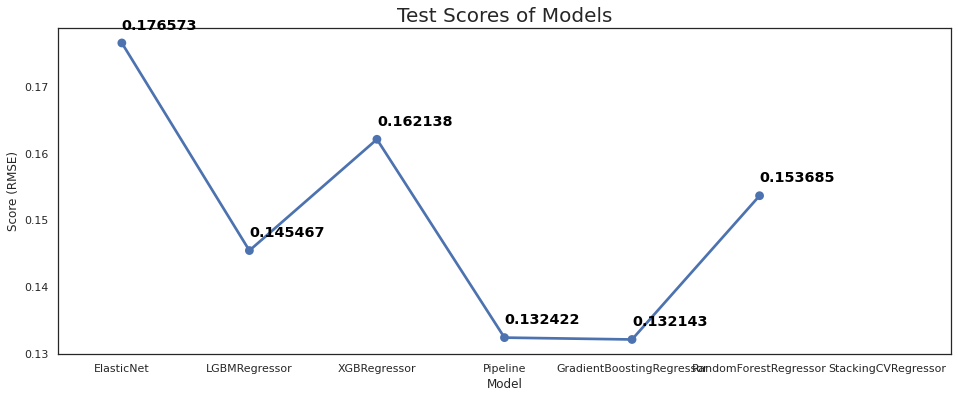
{'ElasticNet': (0.17657340942074354, 0.03990470702503486), 'LGBMRegressor': (0.14546714293442034, 0.03976267856710425), 'XGBRegressor': (0.16213776204326213, 0.02940078347785184), 'Pipeline': (0.13242220591346968, 0.07109241750486699), 'GradientBoostingRegressor': (0.1321431159536556, 0.0387539517785031), 'RandomForestRegressor': (0.15368455919244703, 0.030021849118237243), 'StackingCVRegressor': (nan, nan)}

# Plot the predictions for each model
sns.set_style("white")
fig = plt.figure(figsize=(16, 6))

ax = sns.pointplot(x=list(model_scores.keys()), y=[score for score, _ in model_scores.values()], markers=['o'], linestyles=['-'])
for i, score in enumerate(model_scores.values()):
    ax.text(i, score[0] + 0.002, '{:.6f}'.format(score[0]), horizontalalignment='left', size='large', color='black', weight='semibold')

plt.ylabel('Score (RMSE)')
plt.xlabel('Model')
plt.tick_params(axis='x')
plt.tick_params(axis='y')

plt.title('Test Scores of Models', size=20)

plt.show()

posx and posy should be finite values
posx and posy should be finite values

png

Share on

Twitter Facebook LinkedIn

House Sale Price Prediction

Giao Nguyen-Quynh

Introduction

Data Preprocessing and Exploring

Model Definition

Model Fitting

Share on

You may also enjoy

Create a Stack Bot for Stock Indexes Notification

World Hapiness

Algorithm Visualization Web App with JavaFX, JPro, Docker and Heroku

Detect Covid Infection on X-ray Images with Transfer Learning

	MSZoning_RL	Street_Pave	LotShape_IR1	LotShape_Reg	LandContour_Lvl	Utilities_AllPub	LotConfig_Corner	LotConfig_FR2	LotConfig_Inside	LandSlope_Gtl	Neighborhood_CollgCr	Neighborhood_Crawfor	...	HeatingQC_Ex	HeatingQC_Gd	CentralAir_Y	KitchenQual_Gd	KitchenQual_TA	Functional_Typ	PavedDrive_Y	SaleType_WD	SaleCondition_Abnorml	SaleCondition_Normal
0	1	1	0	1	1	1	0	0	1	1	1	0	...	1	0	1	1	0	1	1	1	0	1
1	1	1	0	1	1	1	0	1	0	1	0	0	...	1	0	1	0	1	1	1	1	0	1
2	1	1	1	0	1	1	0	0	1	1	1	0	...	1	0	1	1	0	1	1	1	0	1
3	1	1	1	0	1	1	1	0	0	1	0	1	...	0	1	1	1	0	1	1	1	1	0
4	1	1	1	0	1	1	0	1	0	1	0	0	...	1	0	1	1	0	1	1	1	0	1

	MSZoning_RL	Street_Pave	LotShape_IR1	LotShape_Reg	LandContour_Lvl	Utilities_AllPub	LotConfig_Corner	LotConfig_FR2	LotConfig_Inside	LandSlope_Gtl	Neighborhood_CollgCr	Neighborhood_Crawfor	...	HeatingQC_Ex	HeatingQC_Gd	CentralAir_Y	KitchenQual_Gd	KitchenQual_TA	Functional_Typ	PavedDrive_Y	SaleType_WD	SaleCondition_Abnorml	SaleCondition_Normal
0	1	1	0	1	1	1	0	0	1	1	1	0	...	1	0	1	1	0	1	1	1	0	1
1	1	1	0	1	1	1	0	1	0	1	0	0	...	1	0	1	0	1	1	1	1	0	1
2	1	1	1	0	1	1	0	0	1	1	1	0	...	1	0	1	1	0	1	1	1	0	1
3	1	1	1	0	1	1	1	0	0	1	0	1	...	0	1	1	1	0	1	1	1	1	0
4	1	1	1	0	1	1	0	1	0	1	0	0	...	1	0	1	1	0	1	1	1	0	1

	MSZoning_RL	Street_Pave	LotShape_IR1	LotShape_Reg	LandContour_Lvl	Utilities_AllPub	LotConfig_Corner	LotConfig_FR2	LotConfig_Inside	LandSlope_Gtl	Neighborhood_CollgCr	Neighborhood_Crawfor	...	HeatingQC_Ex	HeatingQC_Gd	CentralAir_Y	KitchenQual_Gd	KitchenQual_TA	Functional_Typ	PavedDrive_Y	SaleType_WD	SaleCondition_Abnorml	SaleCondition_Normal
0	1	1	0	1	1	1	0	0	1	1	1	0	...	1	0	1	1	0	1	1	1	0	1
1	1	1	0	1	1	1	0	1	0	1	0	0	...	1	0	1	0	1	1	1	1	0	1
2	1	1	1	0	1	1	0	0	1	1	1	0	...	1	0	1	1	0	1	1	1	0	1
3	1	1	1	0	1	1	1	0	0	1	0	1	...	0	1	1	1	0	1	1	1	1	0
4	1	1	1	0	1	1	0	1	0	1	0	0	...	1	0	1	1	0	1	1	1	0	1