Cat Face Generator

Generative networks refer to a class of unsupervised deep learning models that learns the underlying distribution of the data and can generate new data samples. 2 subclasses of generative models are Variational Autoencoder and Generative Adversial Networks. In this blog post, we are going to employ Variational Autoencoder with Convolutional Network to train a deep learning model that learns to generate cat faces. We are building the model with Tensorflow.

from IPython import display

import glob
import imageio
import matplotlib.pyplot as plt
import numpy as np
from PIL import Image
import PIL
import tensorflow as tf
import tensorflow_probability as tfp
import time

batch_size = 64
img_height = 64
img_width = 64

Data Preparation

Let’s prepare the data for training. First of all, download the data from Kaggle and import the image files:

imgs = []
for im_path in glob.glob("cats/*.jpg"):
     img = imageio.imread(im_path)
     img = np.asarray(Image.fromarray(img).resize((img_height, img_width)))
     imgs.append(img)

len(imgs)

15747

all_data = np.asarray(imgs)
all_data.shape, all_data.max(), all_data.min()

((15747, 64, 64, 3), 255, 0)

Visualize some training data:

all_data = (all_data/255).astype('float32')
# print some images
fig = plt.figure(figsize=(16,10))
n_rows = 3
n_cols = 5
for i in range(15):
    plt.subplot(n_rows, n_cols, i + 1)
    plt.imshow(all_data[i])

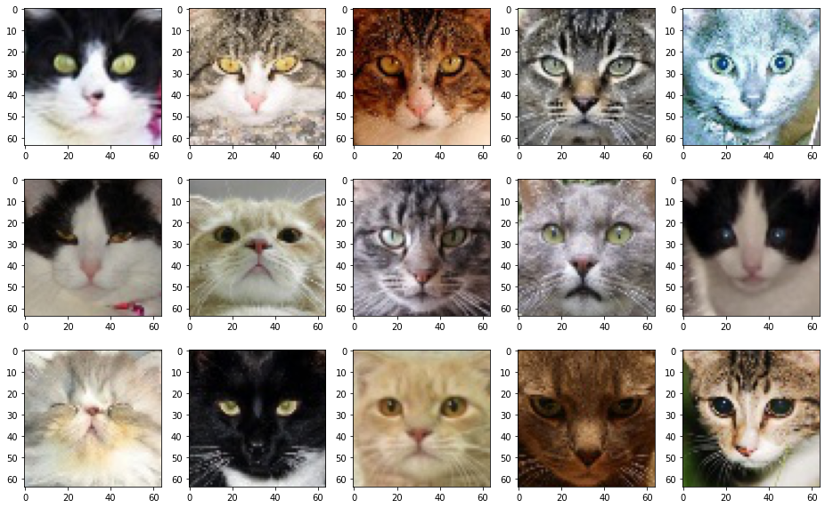
Then split the available dataset in train and test sets:

all_data = np.asarray(imgs)
all_data = (all_data/255).astype('float32')
idx = np.random.permutation(len(all_data))
train_images = all_data[idx[:10000]]
test_images = all_data[idx[10000:]]

The last step is to create the Dataset from image files:

train_dataset = (tf.data.Dataset.from_tensor_slices(train_images).batch(batch_size))
test_dataset = (tf.data.Dataset.from_tensor_slices(test_images).batch(batch_size))

Define models

A traditional autoencoder, which has its origin back to the 1980s is an unsupervised learning technique that attempts to find a good compressed representation of the observations. This technique is deterministic and is trained to reconstruct the input as closely as possible. It works by mapping the observed, potentially high-dimensional data to an unobserved low-dimensional latent space and attempt to reconstruct the observation from the compressed representation. An autoencoder has an hourglass structure to force a useful and compact representation of the observation. Two main components of an autoencoder are its encoder and its decoder. Both components are neural networks. Therefore, they can model arbitrary nonlinear relationship between the involved variables. The task of the encoder is to compress the high-dimensional observations to a potentially lower-dimensional space. The decoder decodes compressed information back into the observation space. The bottleneck architecture avoids that the network learns an identity function. At the same time, it constructs a more condensed latent space.

Variational Autoencoders resemble the structure of autoencoders In general, the VAEs employ two deep neural networks: the generative network, which corresponds to the decoder, maps the latent representation to the observed data; and the inference network, or the encoder, which approximates the posterior that maps the latent space to the observation space. The central objective of VAEs is to find an explicit distribution that can explain the data generation process, instead of learning a deterministic mapping of the data sample to the latent state vector. A VAE is trained to maximize the lower bound on the observations. Please refer to the original paper for more theory detail.

Image from Wikipedia

Since the training data are images, we will use convoluional neural networks for the encoder and decoder.

class CVAE(tf.keras.Model):
  """Convolutional variational autoencoder."""

  def __init__(self, latent_dim = 8):
    super(CVAE, self).__init__()
    self.latent_dim = latent_dim
    self.encoder = tf.keras.Sequential([
            tf.keras.layers.InputLayer(input_shape=(img_height, img_width, 3)),
            tf.keras.layers.Conv2D(
                filters=32, kernel_size=3, strides=(2, 2), activation='relu'),
            tf.keras.layers.Conv2D(
                filters=64, kernel_size=3, strides=(2, 2), activation='relu'),
            tf.keras.layers.Flatten(),
            # No activation
            tf.keras.layers.Dense(latent_dim + latent_dim)])

    self.decoder = tf.keras.Sequential([
            tf.keras.layers.InputLayer(input_shape=(latent_dim,)),
            tf.keras.layers.Dense(units=16*16*32, activation=tf.nn.relu),
            tf.keras.layers.Reshape(target_shape=(16, 16, 32)),
            tf.keras.layers.Conv2DTranspose(
                filters=64, kernel_size=3, strides=2, padding='same',
                activation='relu'),
                
            tf.keras.layers.Conv2DTranspose(
                filters=32, kernel_size=3, strides=2, padding='same',
                activation='relu'),
            # No activation
            tf.keras.layers.Conv2DTranspose(
                filters=3, kernel_size=3, strides=1, padding='same')])

  # sample a single cat image. This is done by choosing a sample from the latent space and
  # project it to the observation space 
  @tf.function
  def sample(self, eps=None):
    if eps is None:
      eps = tf.random.normal(shape=(100, self.latent_dim))
    return self.decode(eps, apply_sigmoid=True)
  # map to the latent space
  def encode(self, x):
    encoded = self.encoder(x)
    mean, logvar = tf.split(encoded, num_or_size_splits=2, axis=1)
    return mean, logvar
  # ensure gradient flow properly
  def reparameterize(self, mean, logvar):
    eps = tf.random.normal(shape=mean.shape)
    return eps * tf.exp(logvar * .5) + mean

  def decode(self, z, apply_sigmoid=False):
    logits = self.decoder(z)
    if apply_sigmoid:
      probs = tf.sigmoid(logits)
      return probs
    return logits

The following code block defines functions to compute the loss:

def compute_loss(model, x):
  mean, logvar = model.encode(x)

  z = model.reparameterize(mean, logvar)

  x_logit = model.decode(z)

  cross_ent = tf.nn.sigmoid_cross_entropy_with_logits(logits=x_logit, labels=x)
  logpx_z = -tf.reduce_sum(cross_ent, axis=[1, 2, 3])
  logpz = log_normal_pdf(z, 0., 0.)
  logqz_x = log_normal_pdf(z, mean, logvar)
  return -tf.reduce_mean(logpx_z + logpz - logqz_x)

Then we define the training loop:

optimizer = tf.keras.optimizers.Adam(1e-3)


def log_normal_pdf(sample, mean, logvar, raxis=1):
  log2pi = tf.math.log(2. * np.pi)
  return tf.reduce_sum(
      -.5 * ((sample - mean) ** 2. * tf.exp(-logvar) + logvar + log2pi),
      axis=raxis)


@tf.function
def train_step(model, x, optimizer):
  """Executes one training step and returns the loss.

  This function computes the loss and gradients, and uses the latter to
  update the model's parameters.
  """
  with tf.GradientTape() as tape:
    loss = compute_loss(model, x)
  gradients = tape.gradient(loss, model.trainable_variables)
  optimizer.apply_gradients(zip(gradients, model.trainable_variables))
  return -loss

Helper function to save intermediate training examples:

def generate_and_save_images(model, epoch, test_sample):
  mean, logvar = model.encode(test_sample)
  z = model.reparameterize(mean, logvar)

  predictions = model.sample(z)
  fig = plt.figure(figsize=(4, 4))

  for i in range(predictions.shape[0]):
    plt.subplot(4, 4, i + 1)
    plt.imshow(predictions[i, :, :])
    plt.axis('off')

  # tight_layout minimizes the overlap between 2 sub-plots
  plt.savefig('image_at_epoch_{:04d}.png'.format(epoch))
  plt.show()

Train the model:

epochs = 38
# set the dimensionality of the latent space to a plane for visualization later
latent_dim = 128
num_examples_to_generate = 16

# Pick a sample of the test set for generating output images
assert batch_size >= num_examples_to_generate
for test_batch in test_dataset.take(1):
  test_sample = test_batch[0:num_examples_to_generate, :, :, :]

random_vector_for_generation = tf.random.normal(
    shape=[num_examples_to_generate, latent_dim])
model = CVAE(latent_dim)
train_hist = []
test_hist = []
generate_and_save_images(model, 0, test_sample)

cur_epoch = 1

for epoch in range(cur_epoch, epochs + 1):
  start_time = time.time()
  for train_x in train_dataset:
    train_elbo = train_step(model, train_x, optimizer)
  end_time = time.time()
  train_hist.append(train_elbo)
  loss = tf.keras.metrics.Mean()
  for test_x in test_dataset:
    loss(compute_loss(model, test_x))
  elbo = -loss.result()
  test_hist.append(elbo)
  display.clear_output(wait=False)
  print('Epoch: {}, Test set ELBO: {}, time elapse for current epoch: {}'
        .format(epoch, elbo, end_time - start_time))
  generate_and_save_images(model, epoch, test_sample)

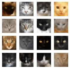
Epoch: 38, Test set ELBO: -6914.81396484375, time elapse for current epoch: 5.114240884780884

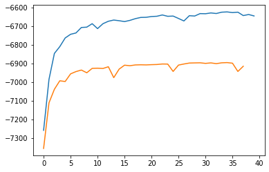
Plot the Evidence Lower Bound over time (negative loss):

plt.plot(train_hist)
plt.plot(test_hist)

[<matplotlib.lines.Line2D at 0x7fe591953e10>]

anim_file = 'cvae.gif'

with imageio.get_writer(anim_file, mode='I') as writer:
  filenames = glob.glob('image*.png')
  filenames = sorted(filenames)
  for filename in filenames:
    image = imageio.imread(filename)
    writer.append_data(image)
  image = imageio.imread(filename)
  writer.append_data(image)

import tensorflow_docs.vis.embed as embed
embed.embed_file(anim_file)

def display_image(epoch_no):
  return PIL.Image.open('image_at_epoch_{:04d}.png'.format(epoch_no))

plt.imshow(display_image(epochs))
plt.axis('off')  # Display images

Model Evaluation

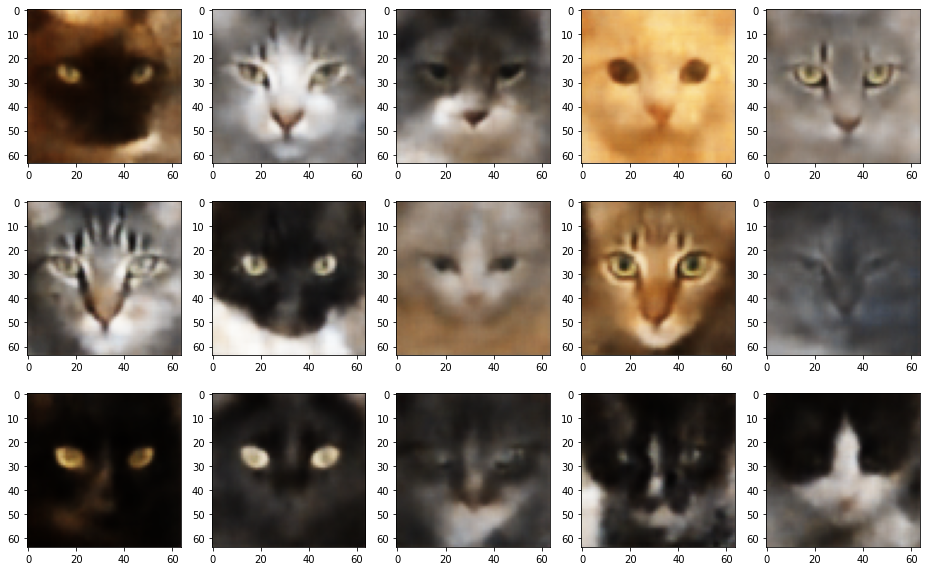
To evaluate the model performance, we check its ability on 2 tasks: generation of new image and reconstruction of real images from the latent encoding:

Test Generation

We sample several images by drawing samples from the latent space and map them onto the images space:

n_rowcol = 6
z = model.reparameterize(np.zeros((n_rowcol * n_rowcol,latent_dim)).astype('float32'), 
                         np.ones((n_rowcol * n_rowcol, latent_dim)).astype('float32'))
predictions = model.sample(z)
fig = plt.figure(figsize=(16, 16))

for i in range(predictions.shape[0]):
  plt.subplot(n_rowcol, n_rowcol, i + 1)
  plt.imshow(predictions[i, :, :])
  plt.axis('off')

  # tight_layout minimizes the overlap between 2 sub-plots
plt.savefig('image_at_epoch_{:04d}.png'.format(epoch))
plt.show()

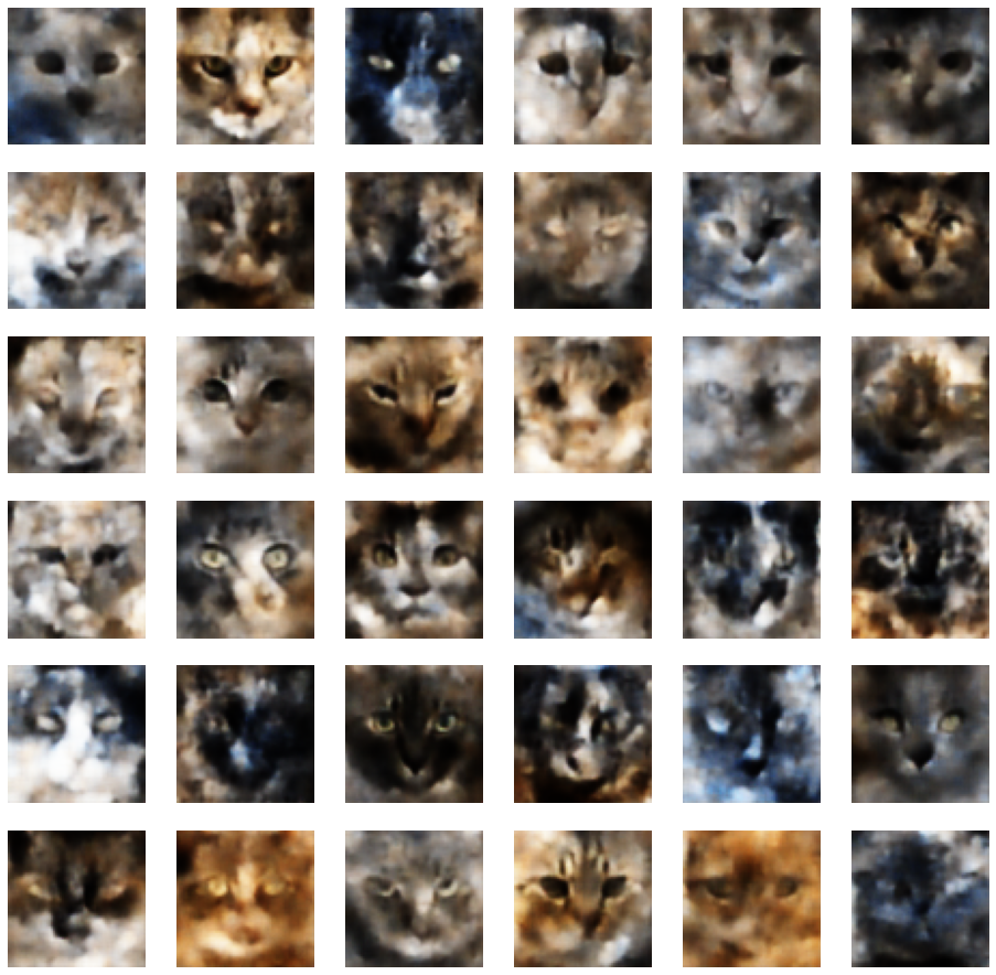
In general, the model has learned the characteristics of a cat face, including the shape, positions of the eyes, nose and plausible feather color.

Test Reconstruction

x = test_images[:15]
mean, logvar = model.encode(x)

z = model.reparameterize(mean, logvar)

x_logit = model.sample(z)

# reconstructed images
fig = plt.figure(figsize=(16,10))
n_rows = 3
n_cols = 5
for i in range(15):
    plt.subplot(n_rows, n_cols, i + 1)
    plt.imshow(x_logit[i] )

# real images
fig = plt.figure(figsize=(16,10))
n_rows = 3
n_cols = 5
for i in range(15):
    plt.subplot(n_rows, n_cols, i + 1)
    plt.imshow(x[i])

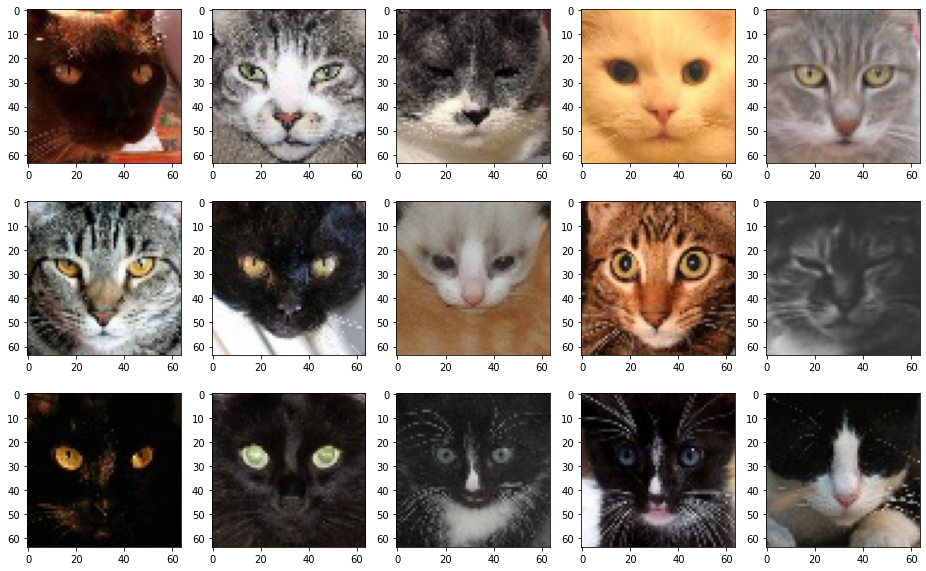
The reconstructed images seem a little blurry, which might lie on our choice of latent space dimension. However, the most important characteristics of the face can be captured.